了解一个算法最好的方法就是实现它,不过在开始实现算法之前,有一些额外的概念需要理解。
Vectorization
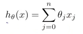
这是上一篇提到的hypothesis的计算公式。
当计算这个表达式值的时候,往往第一个感觉是写一个for loop 然后累加求和
prediction = 0;
for (int i = 0; i < n; ++i) {
    prediction += theta[j] * x[j];
}
但是在machine learning中更倾向于使用矩阵的方式。 比如同样的公式,会看成矩阵相乘。

其中theta和X分别是
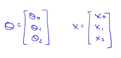
这里通过矩阵或是向量来代替之前的loop。
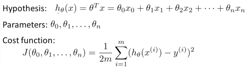
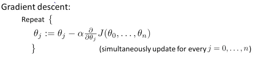
这是上一篇提到的算法
计算function J如果用octave来实现则是这个样子
function J = computeCost(X, y, theta)
%COMPUTECOST Compute cost for linear regression
%   J = COMPUTECOST(X, y, theta) computes the cost of using theta as the
%   parameter for linear regression to fit the data points in X and y

% Initialize some useful values
m = length(y); % number of training examples

% You need to return the following variables correctly
J = 0;

% ====================== YOUR CODE HERE ======================
% Instructions: Compute the cost of a particular choice of theta
%               You should set J to the cost.


t = (X * theta) - y;
J = (sum(t .* t)) / (2 * m);

% =========================================================================

end
而求偏导数迭代更新theta的代码则是这个样子
function [theta, J_history] = gradientDescent(X, y, theta, alpha, num_iters)
%GRADIENTDESCENT Performs gradient descent to learn theta
%   theta = GRADIENTDESENT(X, y, theta, alpha, num_iters) updates theta by
%   taking num_iters gradient steps with learning rate alpha

% Initialize some useful values
m = length(y); % number of training examples
J_history = zeros(num_iters, 1);

for iter = 1:num_iters

    % ====================== YOUR CODE HERE ======================
    % Instructions: Perform a single gradient step on the parameter vector
    %               theta.
    %
    % Hint: While debugging, it can be useful to print out the values
    %       of the cost function (computeCost) and gradient here.
    %


    s = sum(bsxfun(@times, X * theta - y, X));
    theta = theta - (alpha / m) * s';

    % ============================================================

    % Save the cost J in every iteration
    J_history(iter) = computeCost(X, y, theta);

end
上面的2部分代码如果做一些合并分别可以简化成1行代码。说到这里自己还是相当羞愧的。今天早上花了3个小时才搞定这2行代码…主要时间花在了 2个地方。
- 算好theta去predict的上面,和normal equations的方式计算的答案总是对不上,不得不怀疑人生了。。。后面才发现是因为函数没有完全收敛,在调整learning rate之后误差明显变小了。
- 让大脑适应矩阵还是有点难,很多东西看上去很简单,反应很长时间,不过后面会好一些。
为什么用矩阵
在费了老半天力气搞定Vectorization的转变之后,不得不想想为什么要用这个方式做。obviously有2个好处,Andrew课上也提到了好多次。
- 增加一个feature很简单,只要把输入增加一列就好,而算法不需要改动。
- 矩阵的运算更容易优化,性能比循环更快。实际我们往往处理上百万个Example和N多的features
第一个很好理解,而且把循环的一大堆代码写成一行,显得逼格很高。 第二个会比较麻烦,涉及到了并行计算优化。
其他
在之前的算法中,我们看到了每一次调整theta都需要iterate整个所有的example,但实际中往往需要处理上百万个examples,而这样的iteration显然是不能接受的。实际上会随机选取一部分examples然后去迭代theta,最后得到一个较为可靠的theta向量。
最后附上Andrew作业的图片,虽然Andrew 不希望把答案放在网上或是论坛什么的,不过我觉得都过去2年多了,应该没关系了。
 最后的预测效果图
 cost function & theta
 cost function & theta 等高线
 learning rate